This figure is the Fig2 of my research work and I let it rotated.

This time I try o plot the 3d animated distribution via python package Mayavi

Different from the animated operation via using the Matplotlib, This 3d data visualization is more powerful.

I only upload the figure this time and I will write a complete note latterly.

The data are calculated via parameter sweep and store with txt format. We need load it

1
2
3
4
5
6
7
8
9
10
11
12
# %% Load the data
dis_tri = np.loadtxt('../3D_Animation/BigRangeSweep3Cav.txt')
# %%
num_J12 = 199
num_J23 = 200
num_kappa = 201
J12_mat = np.linspace(1, 9, num_J12)
J23_mat = np.linspace(1, 10, num_J23)
kappa_mat = np.linspace(1, 14, num_kappa)

xx, yy, zz = np.mgrid[1:14:201j, 1:10:200j, 1:9:199j]
sym_mat = np.reshape(dis_tri, (num_kappa, num_J23, num_J12))

We need transpose the matrix since I need kappa to be the z axi

1
2
sym_mat_tr = sym_mat.transpose(1, 2, 0)
xx_tr, yy_tr, zz_tr = np.mgrid[1:10:200j, 1:9:199j, 1:14:201j]

Then we can plot the 3d data. The static plot could be plotted first

1
2
3
4
5
6
7
8
9
10
fig_extent = [1, 10, 1, 9, 1, 14]
fig1 = mlab.figure(size=(800, 800), bgcolor=(1, 1, 1), fgcolor=(0, 0, 0))
mlab.contour3d(xx, yy, zz, sym_mat, color=(0, 0.3, 0.3), contours=[
0.8], transparent=True, opacity=0.15) # ,extent=fig_extent)
mlab.contour3d(xx, yy, zz, sym_mat, color=(0, 0.7, 0.7), contours=[
0.9], transparent=True, opacity=0.3) # ,extent=fig_extent)
mlab.contour3d(xx, yy, zz, sym_mat, color=(0, 0, 0.8), contours=[
0.97], transparent=True, opacity=0.4) # ,extent=fig_extent)
mlab.outline(extent=fig_extent)
mlab.axes(color=(1, 0, 0), nb_labels=5)

then we should define a animated function. Since in this case we only need update the view rather than the data. So the code is a little bit diffeent

1
2
3
4
5
6
7
8
9
10
11
12
def make_frame(t):
# camera angle
mlab.view(azimuth=360 * t / duration, elevation=-70, distance=42, focalpoint=[5.5, 5, 7.5])
return mlab.screenshot(antialiased=True)


duration = 5
animation = mpy.VideoClip(make_frame, duration=duration).resize(0.5)
# # Video generation takes 10 seconds, GIF generation takes 25s
# #animation.write_videofile("Rotated_sym_distri_static_Python.mp4", fps=20)
animation.write_gif("Rotated_sym_distri_static_Python.gif", fps=20)
mlab.close(fig1)

The view’s azimuth angle will update each frame. If we want to handle the data, we should use the “mlab.source” to update the arguement as is shown in the offical example

We finally export the gif file and I learned this from this Blog

The figure is a little big and we can compress this gif file in the online web

The following is the figure we obtain

The rotated 3d contour plots