Dipole's Emission In Multi-Layered Structure

Introduction

This is the note of dipole radiation pattern calculations in a multilayer structure.

The numerical realizations can be found in my Github.

The derivations mainly follow the work of Olivier J. F et .al ^ref1

Extra words

My previous calculations are not helpful since we can not get the emission pattern. In previous cylindrical expressions, the integral in has been transformed into Bessel functions via

$$J_{n}(k_{\rho}\rho)=\frac{j^{-n}}{2\pi}\int_{0}^{2\pi}\mathrm{d}k_{\phi}\exp (jk_{\rho}\rho\cos k_\phi)cos(nk_\phi)$$

If we extract the information of , our previous expressions can also be used to get the emission pattern. However, to make this easier to understand, we use plane waves to expand Green’s tensor.

Green tensor expression

We will use Green tensor to get the dipole’s emission!

I will follow the derivations of Paulus et. al . The derivations will begin from the expression of the Green’s tensor. We still consider only the nonmagnetic material so and we use to express the permeability in the vacuum. The equation of the Green’s tensor is as follows

$$\boldsymbol{\nabla}\times\boldsymbol{\nabla}\times \boldsymbol{\overset\leftrightarrow{G}}(\boldsymbol{r},\boldsymbol{r}_0)-k_0^2\varepsilon\mu\boldsymbol{\nabla}\times \boldsymbol{\overset\leftrightarrow{G}}(\boldsymbol{r},\boldsymbol{r}_0)=\boldsymbol{I}\delta(\boldsymbol{r}-\boldsymbol{r}_0)$$

and for a homogeneous media the Green’s tensor can be expressed as

$$\boldsymbol{\overset\leftrightarrow{G}}(\boldsymbol{r},\boldsymbol{r}_0)=\left(1+\frac{\boldsymbol{\nabla}\boldsymbol{\nabla}}{k_B^2}\right)\frac{\exp (jk_BR)}{4\pi R}$$

where $R=|\boldsymbol{R}|=|\boldsymbol{r-r0}|k{B}^2=\omega^2\varepsilon \mu$ corresponds to the wave number in the background medium. We can do Fourier transform of Green’s tensor as

$$\begin{aligned} \boldsymbol{\overset\leftrightarrow{G}}(k)&=\iiint_{-\infty}^{\infty}\boldsymbol{\overset\leftrightarrow{G}}(\boldsymbol{r},\boldsymbol{r}_0)\exp(-j\boldsymbol{k}\cdot\boldsymbol{R})\mathrm{d}\boldsymbol{R}\\ &=\iiint_{-\infty}^{\infty}\left(1+\frac{\boldsymbol{\nabla}\boldsymbol{\nabla}}{k_B^2}\right)\frac{\exp (jk_BR)}{4\pi R} \exp(-j\boldsymbol{k}\cdot\boldsymbol{R})\mathrm{d}\boldsymbol{R}\\ \end{aligned}$$

and we can express the Green’s tensor as a Fourier transform of each wavevector,

$$\boldsymbol{\overset\leftrightarrow{G}}(\boldsymbol{r},\boldsymbol{r}_0)=\frac{1}{8\pi^3k_B^2}\iiint \mathrm{d} \mathbf{k}\left(\frac{\boldsymbol{1}k_B^2-\boldsymbol{\mathrm{k}}\boldsymbol{\mathrm{k}}}{k^2-k_B^2}\right)\exp (j\boldsymbol{\mathrm{k}} \boldsymbol{\cdot R})$$

Since we assume that the layers, which will be added later, are perpendicular to the z axis, we first perform the integration over using calculus of residues. Hence, we muse ensure that the integrand vanishes for and rewrite as

$$\begin{aligned} \mathbf{G}\left(\mathbf{r}, \mathbf{r}_0\right)=& \frac{1}{8 \pi^{3} k_{B}^{2}} \iiint \mathrm{d} \mathbf{k}\left(\frac{\mathbf{1} k_{B}^{2}-\mathbf{k} \mathbf{k}}{k^{2}-k_{B}^{2}}+\hat{\mathbf{z}} \hat{\mathbf{z}}\right) \exp (j \mathbf{k} \cdot \mathbf{R}) \\ &-\frac{\hat{\mathbf{z}} \hat{\mathbf{z}}}{8 \pi^{3} k_{B}^{2}} \iint \mathrm{d} \mathbf{k} \exp (i \mathbf{k} \cdot \mathbf{R}) \\ =& \frac{j}{8 \pi^{2} k_{B}^{2}} \iint \mathrm{d} k_{x} \mathrm{d} k_{y}\left(\frac{\mathbf{1} k_{B}^{2}-\mathbf{k}_{B}\mathbf{k}_{B}}{k_{B z}}\right) \\ & \times \exp \left(j \mathbf{k}_{B} \cdot \mathbf{R}\right)-\frac{\hat{\mathbf{z}} \hat{\mathbf{z}}}{k_{B}^{2}} \delta(\mathbf{R}) \end{aligned}$$

where is the z component of the wave vector and

$$\boldsymbol{\mathrm{k}}_B(k_{Bz})=\left\{ \begin{aligned} k_x\boldsymbol{\hat{x}}+k_y\boldsymbol{\hat{y}}+k_z\boldsymbol{\hat{z}} \quad \text{for} \quad z > z_0,\\ k_x\boldsymbol{\hat{x}}+k_y\boldsymbol{\hat{y}}-k_z\boldsymbol{\hat{z}} \quad \text{for} \quad z < z_0, \end{aligned}\right.$$

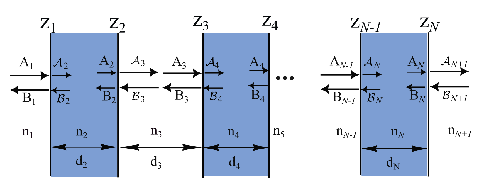
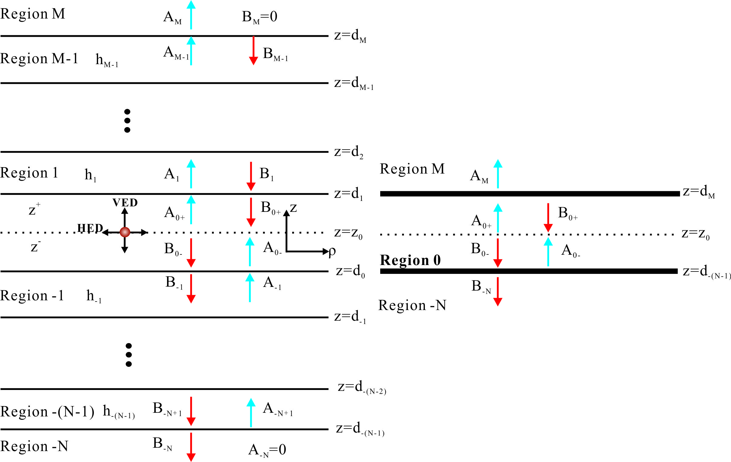
Now that we have the plane-wave expansion of the Green’s tensor for an infinite homogeneous background. It is a simple matter to include additional layers. Indeed, the effect of these layers will be to add two plane waves, one propagating upward and one downward, to each Fourier component, The amplitudes of these additional components are determined by the boundary conditions at the different interfaces. Since the Green’s tensor represents the electric field radiated at by three orthogonal point sources at , the boundary conditions depend on the polarization of the corresponding Fourier component. It is therefore advantageous to introduce a new orthonormal system
$\boldsymbol{\mathrm{\hat{k}}}(k{Bz}),\boldsymbol{\mathrm{\hat{I}}}(k{Bz}),\boldsymbol{\mathrm{\hat{m}}}(k_{Bz})$

$$\boldsymbol{\mathrm{\hat{k}}}(k_{Bz})=\frac{\boldsymbol{\mathrm{k}}(k_{Bz})}{k_B}=(\hat{k}_x(k_{Bz}),\hat{k}_y(k_{Bz}),\hat{k}_z(k_{Bz}))$$ $$\boldsymbol{\mathrm{\hat{I}}}(k_{Bz})=\frac{\boldsymbol{\mathrm{\hat{k}}}(k_{Bz})\times \boldsymbol{\hat{z}}}{|\boldsymbol{\mathrm{\hat{k}}}(k_{Bz})\times \boldsymbol{\hat{z}}|}=(\hat{k}_y(k_{Bz}),-\hat{k}_x(k_{Bz}),0)$$ $$\boldsymbol{\mathrm{\hat{m}}}(k_{Bz})=\boldsymbol{\mathrm{\hat{k}}}(k_{Bz})\times\boldsymbol{\mathrm{\hat{I}}}(k_{Bz})=\left(\hat{k}_x(k_{Bz})\hat{k}_z(k_{Bz}),\hat{k}_y(k_{Bz})\hat{k}_z(k_{Bz}),-\left[\hat{k}_x^2(k_{Bz})+\hat{k}_y^2(k_{Bz})\right]\right)$$

Equivalently, another orthogonal system is formed by $\boldsymbol{\mathrm{\hat{k}}}(-k{Bz}),\boldsymbol{\mathrm{\hat{I}}}(-k{Bz}),\boldsymbol{\mathrm{\hat{m}}}(-k_{Bz})\boldsymbol{\mathrm{\hat{I}}}\boldsymbol{\mathrm{\hat{k}}}\boldsymbol{\mathrm{\hat{z}}}\boldsymbol{\mathrm{\hat{m}}}k_B\boldsymbol{\mathrm{\hat{I}}}\boldsymbol{\mathrm{\hat{m}}}$ corresponds to p polarization, using the fact that

$$\boldsymbol{\mathrm{\hat{k}}}\boldsymbol{\mathrm{\hat{k}}}+\boldsymbol{\mathrm{\hat{I}}}\boldsymbol{\mathrm{\hat{I}}}+\boldsymbol{\mathrm{\hat{m}}}\boldsymbol{\mathrm{\hat{m}}}=\boldsymbol{\mathrm{1}}$$

we can rewrite the Green’s tensor as

$$\mathbf{G}\left(\mathbf{r}, \mathbf{r}^{\prime}\right)=-\frac{\hat{\mathbf{z}} \hat{\mathbf{z}}}{k_{B}^{2}} \delta(\mathbf{R})+\frac{j}{8\pi^2}\iint \mathrm{d} k_{x} \mathrm{d} k_{y}\left(\frac{\boldsymbol{\mathrm{\hat{I}}}\boldsymbol{\mathrm{\hat{I}}}+\boldsymbol{\mathrm{\hat{m}}}\boldsymbol{\mathrm{\hat{m}}}}{k_{Bz}}\right)\times \exp (j\boldsymbol{\mathrm{k}} \boldsymbol{\cdot R})$$

To obtain the Green’s tensor for a stratified medium, we can now superpose to the free-space Green’s tensor of a homogeneous medium the additional terms by formally writing

$$\begin{aligned} \mathbf{G}\left(\mathbf{r}, \mathbf{r}^{\prime}\right)=&-\frac{\hat{\mathbf{z}} \hat{\mathbf{z}}}{k_{l}^{2}} \delta(\mathbf{R})+\frac{i}{8 \pi^{2}} \iint \mathrm{d} k_{x} \mathrm{d} k_{y} \exp \left\{j\left[k_{x}\left(x-x_0\right)+k_{y}\left(y-y_0\right)\right]\right\}\frac{1}{k_{l z}}\\ &\left[\hat{\mathbf{I}}\hat{\mathbf{I}} \exp \left(j k_{l z}\left|z-z_0\right|\right)+\mathbf{R}^{s \uparrow} \exp \left(i k_{l z} z\right)+\mathbf{R}^{s \downarrow} \exp \left(-j k_{l z} z\right)\right.\\ &\left.+\hat{\mathbf{m}}\hat{\mathbf{m}} \exp \left(j k_{l z}\left|z-z_0 \right|\right)+\mathbf{R}^{p \uparrow} \exp \left(i k_{l z} z\right)+\mathbf{R}^{p \downarrow} \exp \left(-j k_{l z} z\right)\right] \end{aligned}$$

where $k{l}^2=\omega^2\varepsilon_l\mu_lk{lz}=\sqrt{kl^2-k_x^2-k_y^2}\mathbf{R}^{s \uparrow},\mathbf{R}^{s \downarrow},\mathbf{R}^{p \uparrow},\mathbf{R}^{p \downarrow}\mathbf{G}\left(\mathbf{r}, \mathbf{r}^{\prime}\right)z>z_0z<z_0A{l,\alpha\beta}^{s/p},B_{l,\alpha\beta}^{s/p}$

$$\begin{aligned} G_{\alpha \beta}\left(\mathbf{r}, \mathbf{r}^{\prime}\right)=& \frac{j}{8 \pi^{2}} \iint \mathrm{d} k_{x} \mathrm{d} k_{y} \exp \left\{j\left[k_{x}\left(x-x^{\prime}\right)\right.\right.\\ &\left.\left.+k_{y}\left(y-y^{\prime}\right)\right]\right\} \frac{1}{k_{l z}}\left\{\left[\hat{l}_{\alpha}\left( \pm k_{l z}\right) A_{l, \alpha \beta}^{s} \exp \left(j k_{l z} z\right)\right.\right.\\ &\left.+\hat{l}_{\alpha}\left(\mp k_{l z}\right) B_{l, \alpha \beta}^{s} \exp \left(-j k_{l z} z\right)\right] \hat{l}_{\beta}\left(k_{l z}\right) \\ &+\left[\hat{m}_{\alpha}\left( \pm k_{l z}\right) A_{l, \alpha \beta}^{p} \exp \left(j k_{l z} z\right)\right.\\ &\left.\left.+\hat{m}_{\alpha}\left(\mp k_{l z}\right) B_{l, \alpha \beta}^{p} \exp \left(-j k_{l z} z\right)\right] \hat{m}_{\beta}\left(k_{l z}\right)\right\} \end{aligned} \label{Galphabeta}$$

We need express each component of the Green’s tensor and then we can write the field distribution for an arbitrary orientate dipole. And the coefficients can be obtained from the outer layer to the emitting layer. It’s necessary for us to write the explict form of the Green tensor. We write the Green tensor as

$$G_{\alpha \beta}\left(\mathbf{r}, \mathbf{r}^{\prime}\right)=\frac{j}{8 \pi^{2}}\iint \mathrm{d} k_{x} \mathrm{d} k_{y} \exp \left\{j\left[k_{x}\left(x-x^{\prime}\right)+k_{y}\left(y-y^{\prime}\right)\right]\right\} \frac{1}{k_{l z}}\left[f_{\alpha,\beta}^s+f_{\alpha,\beta}^p\right]$$

We need write the explicit form of the tensor,

$$1-\boldsymbol{\mathrm{\hat{k}}}\boldsymbol{\mathrm{\hat{k}}}=\frac{1}{k_{l}^{2} }\left[\begin{array}{ccc}{k_{l}^{2}-k_{x}^{2}} & {-k_{x} k_{y}} & {\mp k_{x} k_{lz}} \\ {-k_{x} k_{y}} & {k_{l}^{2}-k_{y}^{2}} & {\mp k_{y} k_{lz}} \\ {\mp k_{x} k_{lz}} & {\mp k_{y} k_{lz}} & {k_{l}^{2}-k_{lz}^{2}}\end{array}\right]$$

and

$$\boldsymbol{\mathrm{\hat{I}}}\boldsymbol{\mathrm{\hat{I}}}=\frac{1}{\left(k_{x}^{2}+k_{y}^{2}\right)}\left[\begin{array}{ccc}{k_{y}^{2}} & {-k_{x} k_{y}} & {0} \\ {-k_{x} k_{y}} & {k_{x}^{2}} & {0} \\ {0} & {0} & {0}\end{array}\right]$$ $$\boldsymbol{\mathrm{\hat{m}}}\boldsymbol{\mathrm{\hat{m}}}=\frac{1}{k_{l}^{2}\left(k_{x}^{2}+k_{y}^{2}\right)}\left[\begin{array}{ccc}{k_{x}^{2} k_{lz}^2} & {k_{x} k_{y} k_{lz}^2} & {\mp k_{x}k_{lz}\left(k_{x}^{2}+k_{y}^{2}\right)} \\ {k_{x} k_{y} k_{lz}^2} & {k_{y}^{2} k_{lz}^2} & {\mp k_{lz}k_{y}\left(k_{x}^{2}+k_{y}^{2}\right)} \\ {\mp k_{x}k_{lz}\left(k_{x}^{2}+k_{y}^{2}\right)} & {\mp k_{lz} k_{y}\left(k_{x}^{2}+k_{y}^{2}\right)} & {\left(k_{x}^{2}+k_{y}^{2}\right)^{2}}\end{array}\right]$$

Since the definition in the [] let the sign attached to $Al,B{l}$, then

$$\boldsymbol{f^s}=\frac{1}{\left(k_{x}^{2}+k_{y}^{2}\right)}\left[\begin{array}{ccc}{k_{y}^{2}} & {-k_{x} k_{y}} & {0} \\ {-k_{x} k_{y}} & {k_{x}^{2}} & {0} \\ {0} & {0} & {0}\end{array}\right]\odot \left(\boldsymbol{A}_{l}^s\exp(jk_{lz}z))+\boldsymbol{B}_{l}^s\exp(-jk_{lz}z)\right)$$ $$\begin{aligned} \boldsymbol{f^p}&=\frac{1}{k_{l}^{2}\left(k_{x}^{2}+k_{y}^{2}\right)}\left[\begin{array}{ccc}{\pm k_{x}^{2} k_{lz}^2} & \pm {k_{x} k_{y} k_{lz}^2} & \mp{k_{x}k_{lz}\left(k_{x}^{2}+k_{y}^{2}\right)} \\ \pm {k_{x} k_{y} k_{lz}^2} & \pm {k_{y}^{2} k_{lz}^2} & \mp{ k_{y}k_{lz}\left(k_{x}^{2}+k_{y}^{2}\right)} \\ { - k_{x}k_{lz}\left(k_{x}^{2}+k_{y}^{2}\right)} & - { k_{y}k_{lz}\left(k_{x}^{2}+k_{y}^{2}\right)} & {\left(k_{x}^{2}+k_{y}^{2}\right)^{2} }\end{array}\right]\odot \boldsymbol{A}_{l}^p\exp(jk_{lz}z))\\ &+\frac{1}{k_{l}^{2}\left(k_{x}^{2}+k_{y}^{2}\right)}\left[\begin{array}{ccc}{\mp k_{x}^{2} k_{lz}^2} & \mp {k_{x} k_{y} k_{lz}^2} & \pm{k_{x}k_{lz}\left(k_{x}^{2}+k_{y}^{2}\right)} \\ \mp {k_{x} k_{y} k_{lz}^2} & \mp {k_{y}^{2} k_{lz}^2} & \pm{ k_{y}k_{lz}\left(k_{x}^{2}+k_{y}^{2}\right)} \\ { - k_{x}k_{lz}\left(k_{x}^{2}+k_{y}^{2}\right)} & - { k_{y}k_{lz}\left(k_{x}^{2}+k_{y}^{2}\right)} & {\left(k_{x}^{2}+k_{y}^{2}\right)^{2} }\end{array}\right]\odot \boldsymbol{B}_{l}^p\exp(-jk_{lz}z) \end{aligned}$$

Here means the multiply of the corresponding elements in each matrix. We now need calculate the accurate expression of the $A{\alpha,\beta}^{s/p},A{\alpha,\beta}^{s/p}A{\alpha,\beta}^{s/p},A{\alpha,\beta}^{s/p}\beta \neq z$

$$A_{0,\alpha \beta}^{p\uparrow/\downarrow}=\pm R^{p\downarrow}_{0,\alpha\beta}\frac{R^{p\uparrow}_{0,\alpha\beta}\exp(-jk_{0z}z_0)-\exp(jk_{0z}z_0)}{1-R^{p\downarrow}_{0,\alpha\beta}R^{p\uparrow}_{0,\alpha\beta}}\pm\Theta(z-z_0)\exp(-jk_{0z}z_0)$$ $$B_{l,\alpha \beta}^{p\uparrow/\downarrow}=\mp R^{p\uparrow}_{0,\alpha\beta}\frac{R^{p\downarrow}_{0,\alpha\beta}\exp(jk_{0z}z_0)-\exp(-jk_{0z}z_0)}{1-R^{p\downarrow}_{0,\alpha\beta}R^{p\uparrow}_{0,\alpha\beta}}\mp \Theta(z_0-z)\exp(jk_{0z}z_0)$$

with

$$A_{l,\alpha \beta}^{p\uparrow/\downarrow}= R^{p\downarrow}_{0,\alpha\beta}\frac{R^{p\uparrow}_{0,\alpha\beta}\exp(-jk_{0z}z_0)+\exp(jk_{0z}z_0)}{1-R^{p\downarrow}_{0,\alpha\beta}R^{p\uparrow}_{0,\alpha\beta}}+\Theta(z-z_0)\exp(-jk_{0z}z_0)$$ $$B_{l,\alpha \beta}^{p\uparrow/\downarrow}= R^{p\uparrow}_{0,\alpha\beta}\frac{R^{p\downarrow}_{0,\alpha\beta}\exp(jk_{0z}z_0)+\exp(-jk_{0z}z_0)}{1-R^{p\downarrow}_{0,\alpha\beta}R^{p\uparrow}_{0,\alpha\beta}}+ \Theta(z_0-z)\exp(jk_{0z}z_0)$$

For the s polarization

$$A_{l,\alpha \beta}^{s\uparrow/\downarrow}= R^{s\downarrow}_{0,\alpha\beta}\frac{R^{s\uparrow}_{0,\alpha\beta}\exp(-jk_{0z}z_0)+\exp(jk_{0z}z_0)}{1-R^{s\downarrow}_{0,\alpha\beta}R^{s\uparrow}_{0,\alpha\beta}}+\Theta (z-z_0)\exp(-jk_{0z}z_0)$$ $$B_{l,\alpha \beta}^{s\uparrow/\downarrow}= R^{s\uparrow}_{0,\alpha\beta}\frac{R^{s\downarrow}_{0,\alpha\beta}\exp(jk_{0z}z_0)+\exp(-jk_{0z}z_0)}{1-R^{s\downarrow}_{0,\alpha\beta}R^{s\uparrow}_{0,\alpha\beta}}+ \Theta (z_0-z)\exp(jk_{0z}z_0)$$

In above expressions, are the total reflections in the emitting layer, we define the reflection coefficients in the upper space for each interface as

$$R_{l,\alpha\beta}^{p\uparrow}=\frac{B_{l,\alpha\beta}^{p\uparrow}}{A_{l,\alpha\beta}^{p\uparrow}},R_{l,\alpha\beta}^{s\uparrow}=\frac{B_{l,\alpha\beta}^{s\uparrow}}{A_{l,\alpha\beta}^{s\uparrow}}$$

the same with the lower space

$$R_{l}^{p\downarrow}=\frac{A_{l}^{p\downarrow}}{B_{l}^{p\downarrow}},R_{l}^{s\downarrow}=\frac{A_{l}^{s\downarrow}}{B_{l}^{s\downarrow}}$$

the reflections can be calculated iteratively from the outer layer

$$R_{l,\alpha\beta}^{s/p,\uparrow}=\frac{R_{l+1,\alpha\beta}^{s/p,\uparrow}e^{-j(k_{(l+1)z}-k_{lz})d_{l+1}}+R_{l(l+1)}^{s/p}e^{j(k_{(l+1)z}+k_{lz})d_{l+1}}}{R_{l+1,\alpha\beta}^{s/p,\uparrow}R_{l(l+1)}^{s/p}e^{-j(k_{(l+1)z}+k_{lz})d_{l+1}}+e^{j(k_{(l+1)z}-k_{lz})d_{l+1}}}$$ $$R_{l,\alpha\beta}^{s/p,\downarrow}=\frac{R_{l-1,\alpha\beta}^{s/p,\downarrow}e^{j(k_{(l-1)z}-k_{lz})d_{l}}+R_{l(l-1)}^{s/p}e^{-j(k_{(l-1)z}+k_{lz})d_{l}}}{R_{l-1,\alpha\beta}^{s/p,\downarrow}R_{l(l-1)}^{s/p}e^{j(k_{(l-1)z}+k_{lz})d_{l}}+e^{-j(k_{(l-1)z}-k_{lz})d_{l}}}$$

where

$$R_{l(l-1)}^{p}=\frac{\varepsilon_{l-1} k_{l z}-\varepsilon_{l} k_{l-1, z}}{\varepsilon_{l} k_{(l-1) z}+\varepsilon_{l-1} k_{l z}}=-R_{(l-1) l}^{p} \quad R_{l(l-1)}^{s}=\frac{k_{l z}-k_{(l-1) z}}{k_{(l-1) z}+k_{l z}}=-R_{(l-1) l}^{s}$$

and

$$T_{l(l-1)}^{p}=\frac{2\varepsilon_{l-1} k_{l z}}{\varepsilon_{l} k_{(l-1) z}+\varepsilon_{l-1} k_{l z}}=1+R_{l(l-1) }^{p} \quad T_{l(l-1)}^{s}=\frac{2k_{l z}}{k_{(l-1) z}+k_{l z}}=1+R_{l(l-1)}^{s}$$

So we can calculate the coefficients in the emitting layer, and the coefficients in other can be calculated via the transmission matrix.

In the upper space

$$A_{l+1,\alpha\beta}^{s/p}=\gamma^{s/p}\left[A_{l,\alpha\beta}^{s/p}e^{j(k_{lz}-k_{(l+1)z})d_{l+1}}+R_{(l+1)l}^{s/p}B_{l,\alpha\beta}^{s/p} e^{-j(k_{lz}+k_{(l+1)z})d_{l+1}}\right]$$ $$B_{l+1,\alpha\beta}^{s/p}=\gamma^{s/p}\left[R_{(l+1)l}^{s/p}A_{l,\alpha\beta}^{s/p}e^{j(k_{lz}+k_{(l+1)z})d_{l+1}}+B_{l,\alpha\beta}^{s/p} e^{-j(k_{lz}-k_{(l+1)z})d_{l+1}}\right]$$

where

$$\gamma^{s}=\frac{1}{2}\frac{k_{lz}+k_{(l+1)z}}{k_{lz}}=\frac{1}{1-R^{s}_{(l+1)l}}$$ $$\gamma^{p}=\frac{1}{2}\frac{k_{lz}\varepsilon_{l+1}+\varepsilon_{l}k_{(l+1)z}}{k_{(l+1)z}\varepsilon_{l}}=\frac{1}{1+R^{p}_{(l+1)l}},\quad \text {for } \quad \beta=x,y,\quad\alpha=x,y,z$$ $$\gamma^{p}=\frac{1}{2}\frac{k_{lz}\varepsilon_{l+1}+\varepsilon_{l}k_{lz}}{k_{lz}\varepsilon_{l+1}}=\frac{k_{(l+1)z}}{k_{lz}}\frac{1}{1+R^{p}_{(l+1)l}},\quad \text {for } \quad \beta=z, \quad\alpha=x,y,z$$

In the lower space

$$A_{l-1,\alpha\beta}^{s/p}=\gamma^{s/p}\left[A_{l,\alpha\beta}^{s/p}e^{j(k_{lz}-k_{(l-1)z})d_{l}}+R_{(l-1)l}^{s/p}B_{l,\alpha\beta}^{s/p} e^{-j(k_{lz}+k_{(l-1)z})d_{l}}\right]$$ $$B_{l-1,\alpha\beta}^{s/p}=\gamma^{s/p}\left[R_{(l-1)l}^{s/p}A_{l,\alpha\beta}^{s/p}e^{j(k_{lz}+k_{(l-1)z})d_{l}}+B_{l,\alpha\beta}^{s/p} e^{-j(k_{lz}-k_{(l-1)z})d_{l}}\right]$$

where

$$\gamma^{s}=\frac{1}{2}\frac{k_{lz}+k_{(l-1)z}}{k_{lz}}=\frac{1}{1-R^{s}_{(l-1)l}}$$ $$\gamma^{p}=\frac{1}{2}\frac{k_{lz}\varepsilon_{l-1}+\varepsilon_{l}k_{(l-1)z}}{k_{(l-1)z}\varepsilon_{l}}=\frac{1}{1+R^{p}_{(l-1)l}},\quad \text {for } \quad \beta=x,y,\quad\alpha=x,y,z$$ $$\gamma^{p}=\frac{1}{2}\frac{k_{lz}\varepsilon_{l-1}+\varepsilon_{l}k_{(l-1)z}}{k_{lz}\varepsilon_{l}}=\frac{k_{(l-1)z}}{k_{lz}}\frac{1}{1+R^{p}_{(l-1)l}},\quad \text {for } \quad \beta=z, \quad\alpha=x,y,z$$

The field expression and emission pattern

The Green’s tensor can be obtained in previous section, the electric field and magnetic field can be obtained from the Green’s tensor via

$$\vec{E}(r)=j\omega\mu_0 \boldsymbol{\overset\leftrightarrow{G}}(\boldsymbol{r},\boldsymbol{r}_0)\boldsymbol{p}=j\omega\mu_0 \left(\boldsymbol{\overset\leftrightarrow{I}}+\frac{\nabla \nabla}{k^{2}}\right) G_0(\boldsymbol{r},\boldsymbol{r}_0)\boldsymbol{p}$$ $$\vec{H}(r)=\nabla \times \left(\boldsymbol{\overset\leftrightarrow{G}}(\boldsymbol{r},\boldsymbol{r}_0)\boldsymbol{p}\right)=\nabla \times \left(\boldsymbol{\overset\leftrightarrow{I}}+\frac{\nabla \nabla}{k^{2}}\right) G_0(\boldsymbol{r},\boldsymbol{r}_0)\boldsymbol{p}=\nabla \times G_0(\boldsymbol{r},\boldsymbol{r}_0)\boldsymbol{p}$$

And we can write the electric field as

$$E(r)=\iint \boldsymbol{E}^{s}(k_x,k_y,k_z)+\boldsymbol{E}^{p}(k_x,k_y,k_z)\mathrm{d}k_x\mathrm{d}k_y$$

The far field observed in the direction of the dimensionless unit vector

$$\boldsymbol{s}=(s_x,s_y,s_z)=(\boldsymbol{\frac{x}{r}},\boldsymbol{\frac{y}{r}},\boldsymbol{\frac{z}{r}})=(\frac{k_x}{k},\frac{k_y}{k},\frac{k_z}{k})$$

is determined by the Fourier spectrum as as

$$\boldsymbol{E}_{\infty}(s_x,s_y)=-iks_z \boldsymbol{E}(ks_x,ks_y;0)\frac{e^{ikr}}{r}$$

In the far field , the magnetic field vector is transverse to the electric field vector and the time-averaged Poynting vectors is
calculated as

$$\langle \boldsymbol{S}\rangle =\frac{1}{2}\text{Re}\{\boldsymbol{E}\times \boldsymbol{H}\}=\frac{1}{2}\sqrt{\frac{\epsilon_0\varepsilon_l}{\mu_0\mu_l}}(\boldsymbol{E}\cdot \boldsymbol{E}^{*})\cdot\boldsymbol{n}_{r}$$

Since the s and p polarized field are orthogonal, then we can express the far field power as

$$\begin{aligned} &\iint \frac{1}{2}\sqrt{\frac{\epsilon_0\varepsilon_l}{\mu_0\mu_l}}(\boldsymbol{E_{\infty}}\cdot \boldsymbol{E_{\infty}}^{*})\cdot\boldsymbol{n}_{r}\cdot r^2\sin\theta \mathrm{d}\theta \mathrm{d}\phi\\ =&\iint \frac{1}{2}\sqrt{\frac{\epsilon_0\varepsilon_l}{\mu_0\mu_l}}k_z^2 |\boldsymbol{E}(ks_x,ks_y;0)\cdot\boldsymbol{n}_{r}|^2 \cdot \sin\theta \mathrm{d} \theta \mathrm{d}\phi\\ =& \frac{1}{2}\sqrt{\frac{\epsilon_0\varepsilon_l}{\mu_0\mu_l}}\iint \left(|\boldsymbol{E}|^2_s+|\boldsymbol{E}|^2_p \right)k^2\cos^2\theta \cdot \mathrm{d}\Omega\\ =& \iint I(\theta,\phi)\mathrm{d}\Omega \end{aligned}$$

where the emission pattern is

$$I(\theta,\phi)=\frac{1}{2}\sqrt{\frac{\epsilon_0\varepsilon_l}{\mu_0\mu_l}}\left(|\boldsymbol{E}|^2_s+|\boldsymbol{E}|^2_p \right)k^2\cos^2\theta$$

Numerical Implementation

Our previous expressions are not suitable for numerical implementation since there are maximum numbers in the exponent. To let is more applicable we rewrite the expressions. We define in the upper space

$$\widehat{A}_{l,\alpha\beta}^{s/p}=A_{l,\alpha\beta}^{s,p}\exp(jk_{lz}d_{l+1}),\quad \widehat{B}_{l,\alpha\beta}^{s/p}=B_{l,\alpha\beta}^{s,p}\exp(-jk_{lz}d_{l+1})$$

and in the lower space

$$\widehat{A}_{l,\alpha\beta}^{s/p}=A_{l,\alpha\beta}^{s,p}\exp(jk_{lz}d_{l}),\quad \widehat{B}_{l,\alpha\beta}^{s/p}=B_{l,\alpha\beta}^{s,p}\exp(-jk_{lz}d_{l})$$

If we use these expression, The green tensor should be

$$\begin{equation} \begin{aligned} G_{\alpha \beta}\left(\mathbf{r}, \mathbf{r}^{\prime}\right)=& \frac{j}{8 \pi^{2}} \iint \mathrm{d} k_{x} \mathrm{d} k_{y} \exp \left\{j\left[k_{x}\left(x-x^{\prime}\right)\right.\right. \\ &\left.\left.+k_{y}\left(y-y^{\prime}\right)\right]\right\} \frac{1}{k_{l z}}\left\{\left[\hat{l}_{\alpha}\left( \pm k_{l z}\right) \widehat{A}_{l, \alpha \beta}^{s} \exp \left(j k_{l z} (z-z_{l})\right)\right.\right. \\ &\left.+\hat{l}_{\alpha}\left(\mp k_{l z}\right) \widehat{B}_{l, \alpha \beta}^{s} \exp \left(-j k_{l z} (z-z_{l})\right)\right] \hat{l}_{\beta}\left(k_{l z}\right) \\ &+\left[\hat{m}_{\alpha}\left( \pm k_{l z}\right) \widehat{A}_{l, \alpha \beta}^{p} \exp \left(j k_{l z} (z-z_{l})\right)\right.\\ &\left.\left.+\hat{m}_{\alpha}\left(\mp k_{l z}\right) \widehat{B}_{l, \alpha \beta}^{p} \exp \left(-j k_{l z} (z-z_{l})\right)\right] \hat{m}_{\beta}\left(k_{l z}\right)\right\} \end{aligned} \end{equation}$$

where $z{l}=d{l+1}z>z0z{l}=d_{l}z<z_0$. The coefficients relation between different layers can be rewritten as

In the upper space

$$\widehat{A}_{l+1,\alpha\beta}^{s/p}=\gamma^{s/p}\left[\widehat{A}_{l,\alpha\beta}^{s/p}e^{jk_{lz}(d_{l+1}-d_{l})}+R_{(l+1)l}^{s/p}\widehat{B}_{l,\alpha\beta}^{s/p} e^{-jk_{lz}(d_{l+1}-d_{l})}\right]$$ $$\widehat{B}_{l+1,\alpha\beta}^{s/p}=\gamma^{s/p}\left[R_{(l+1)l}^{s/p}\widehat{A}_{l,\alpha\beta}^{s/p}e^{jk_{lz}(d_{l+1}-d_{l})}+\widehat{B}_{l,\alpha\beta}^{s/p}e^{-jk_{lz}(d_{l+1}-d_{l})}\right]$$

where

$$\gamma^{s}=\frac{1}{2}\frac{k_{lz}+k_{(l+1)z}}{k_{lz}}=\frac{1}{1-R^{s}_{(l+1)l}}$$ $$\gamma^{p}=\frac{1}{2}\frac{k_{lz}\varepsilon_{l+1}+\varepsilon_{l}k_{(l+1)z}}{k_{(l+1)z}\varepsilon_{l}}=\frac{1}{1+R^{p}_{(l+1)l}},\quad \text {for } \quad \beta=x,y,\quad\alpha=x,y,z$$ $$\gamma^{p}=\frac{1}{2}\frac{k_{lz}\varepsilon_{l+1}+\varepsilon_{l}k_{lz}}{k_{lz}\varepsilon_{l+1}}=\frac{k_{(l+1)z}}{k_{lz}}\frac{1}{1+R^{p}_{(l+1)l}},\quad \text {for } \quad \beta=z, \quad\alpha=x,y,z$$

In the lower space

$$\widehat{A}_{l-1,\alpha\beta}^{s/p}=\gamma^{s/p}\left[\widehat{A}_{l,\alpha\beta}^{s/p}e^{jk_{lz}(d_{l}-d_{l-1})}+R_{(l-1)l}^{s/p}\widehat{B}_{l,\alpha\beta}^{s/p} e^{-jk_{lz}(d_{l}-d_{l-1})}\right]$$ $$\widehat{B}_{l-1,\alpha\beta}^{s/p}=\gamma^{s/p}\left[R_{(l-1)l}^{s/p}\widehat{A}_{l,\alpha\beta}^{s/p}e^{jk_{lz}(d_{l}-d_{l-1})}+\widehat{B}_{l,\alpha\beta}^{s/p} e^{-jk_{lz}(d_{l}-d_{l-1})}\right]$$

where

$$\gamma^{s}=\frac{1}{2}\frac{k_{lz}+k_{(l-1)z}}{k_{lz}}=\frac{1}{1-R^{s}_{(l-1)l}}$$ $$\gamma^{p}=\frac{1}{2}\frac{k_{lz}\varepsilon_{l-1}+\varepsilon_{l}k_{(l-1)z}}{k_{(l-1)z}\varepsilon_{l}}=\frac{1}{1+R^{p}_{(l-1)l}},\quad \text {for } \quad \beta=x,y,\quad\alpha=x,y,z$$ $$\gamma^{p}=\frac{1}{2}\frac{k_{lz}\varepsilon_{l-1}+\varepsilon_{l}k_{(l-1)z}}{k_{lz}\varepsilon_{l}}=\frac{k_{(l-1)z}}{k_{lz}}\frac{1}{1+R^{p}_{(l-1)l}},\quad \text {for } \quad \beta=z, \quad\alpha=x,y,z$$

Relations of amplitudes in different layers

In this section , I will complete the derivations of the relations of in different layers. The boundary conditions in each interface can be written as

$$\widehat{z}\times\left(\mathbf{G}^{+}-\mathbf{G}^{-}\right)=\mathbf{0}$$ $$\widehat{z}\cdot\left(\boldsymbol{\varepsilon}^{+} \mathbf{G}^{+}-\boldsymbol{\varepsilon}^{-}\mathbf{G}^{-}\right)=\mathbf{0}$$ $$\widehat{z}\times\mathbf{\nabla}\times \left(\frac{\mathbf{G}^{+}}{\mu_+}-\frac{\mathbf{G}^{-}}{\mu_{-}}\right)=\mathbf{0}$$ $$\widehat{z}\cdot\mathbf{\nabla} \times\left(\mathbf{G}^{+}-\mathbf{G}^{-}\right)=\mathbf{0}$$

For convenience we need write the Green’s tensor into a more simple from which can be used to express the boundary conditions. We can express the total green tensor as

$$\mathbf{G}=\frac{j}{8 \pi^{2}}\iint \mathrm{d} k_{x} \mathrm{d} k_{y} \exp \left\{j\left[k_{x}\left(x-x^{\prime}\right)+k_{y}\left(y-y^{\prime}\right)\right]\right\}\left[F_{A}\odot A \cdot e^{jk_{lz}z}+F_{B}\odot B \cdot e^{-jk_{lz}z}\right]$$

where $F{A/B}k{lz},k{l}F{A/B}$ in a more simple form as

$$F_{A/B}=U_{A/B}\cdot V_{A/B}$$

where $U{A/B}k{lz},\varepsilon$. We write the explicit form for each as follows.

S polarized light upper/lower layer

$$U_{A/B}^{s\uparrow\downarrow}=\frac{1}{\left(k_{x}^{2}+k_{y}^{2}\right)}\left[\begin{array}{ccc}{k_{y}^{2}} & {-k_{x} k_{y}} & {0} \\ {-k_{x} k_{y}} & {k_{x}^{2}} & {0} \\ {0} & {0} & {0}\end{array}\right],V_{A/B}^{s\uparrow\downarrow}=\left[\begin{array}{ccc}{1} & {1} & {1} \\ {1} & {1} & {1}\\ {1} & {1} & {1}\end{array}\right]\frac{1}{k_{lz}}$$

P polarized light upper/lower layer

$$\begin{aligned} U_{A}^{p\uparrow\downarrow}&=\frac{1}{\left(k_{x}^{2}+k_{y}^{2}\right)}\left[\begin{array}{ccc}{\pm k_{x}^{2} } & \pm {k_{x} k_{y} } & \mp{k_{x}\left(k_{x}^{2}+k_{y}^{2}\right)} \\ \pm {k_{x} k_{y} } & \pm {k_{y}^{2} } & \mp{ k_{y}\left(k_{x}^{2}+k_{y}^{2}\right)} \\ { - k_{x}\left(k_{x}^{2}+k_{y}^{2}\right)} & - { k_{y}\left(k_{x}^{2}+k_{y}^{2}\right)} & {\left(k_{x}^{2}+k_{y}^{2}\right)^{2} }\end{array}\right]\\ U_{B}^{p\uparrow\downarrow}&=\frac{1}{\left(k_{x}^{2}+k_{y}^{2}\right)}\left[\begin{array}{ccc}{\pm k_{x}^{2} } & \pm {k_{x} k_{y} } & \mp{k_{x}\left(k_{x}^{2}+k_{y}^{2}\right)} \\ \pm {k_{x} k_{y} } & \pm {k_{y}^{2} } & \mp{ k_{y}\left(k_{x}^{2}+k_{y}^{2}\right)} \\ { - k_{x}\left(k_{x}^{2}+k_{y}^{2}\right)} & - { k_{y}\left(k_{x}^{2}+k_{y}^{2}\right)} & {\left(k_{x}^{2}+k_{y}^{2}\right)^{2} }\end{array}\right]\\ \end{aligned}$$ $$\begin{aligned} V_{A}^{p\uparrow\downarrow}&=\frac{1}{k_{l}^{2}k_{lz}}\left[\begin{array}{ccc}{ k_{lz}^2} & {k_{lz}^2} & k_{lz} \\ k_{lz}^2 & k_{lz}^2 & k_{lz} \\ k_{lz} & k_{lz} & 1 \end{array}\right]\\ V_{B}^{p\uparrow\downarrow}&=\frac{1}{k_{l}^{2}k_{lz}}\left[\begin{array}{ccc}{ -k_{lz}^2} & -{k_{lz}^2} & -k_{lz} \\ -k_{lz}^2 & -k_{lz}^2 & -k_{lz} \\ k_{lz} & k_{lz} & 1 \end{array}\right]\\ \end{aligned}$$

Then in deriving the relations of coefficients between different layers, we can only use

$$\boldsymbol{G}^{'}=V_{A}^{s/p,\uparrow\downarrow} A^{s/p,\uparrow\downarrow} e^{jk_{lz}z}+V_{B}^{s/p,\uparrow\downarrow} B^{s/p,\uparrow\downarrow} e^{jk_{lz}z}$$

which is more convenient to write. For convenience, we could also write the Green’s tensor as

$$\boldsymbol{G}=[\boldsymbol{G}_{1},\boldsymbol{G}_{2},\boldsymbol{G}_{3}]$$

so that the boundary conditions can be written as

$$[-(\boldsymbol{G}^{+}_{2i}-\boldsymbol{G}^{-}_{2i}),(\boldsymbol{G}^{+}_{1i}-\boldsymbol{G}^{-}_{1i}),0]^T=0 \label{eq75}$$ $$[0,0,(\varepsilon^{+}\boldsymbol{G}^{+}_{3i}-\varepsilon^{-}\boldsymbol{G}^{-}_{3i})]^{T}=0 \label{eq76}$$ $$\left[-(\partial_z (\boldsymbol{G}_{1i}^{+}/\mu_{+}-\boldsymbol{G}_{1i}^{-}/\mu_{-})-\partial_x (\boldsymbol{G}_{3i}^{+}/\mu_{+}-\boldsymbol{G}_{3i}^{-}/\mu_{-})),\partial_y (\boldsymbol{G}_{3i}^{+}/\mu_{+}-\boldsymbol{G}_{3i}^{-}/\mu_{-})-\partial_z (\boldsymbol{G}_{2i}^{+}/\mu_{+}-\boldsymbol{G}_{2i}^{-}/\mu_{-}),0\right]^T=0 \label{eq77}$$ $$\left[0,0,\partial_x (\boldsymbol{G}_{2i}^{+}-\boldsymbol{G}_{2i}^{-})-\partial_y (\boldsymbol{G}_{1i}^{+}-\boldsymbol{G}_{1i}^{-})\right]^T=0 \label{eq78}$$

Then

$$(F_{A2i}^{+}A^{+}_{2i}e^{ik_{z}^{+}z_{0}}+F_{B2i}^{+}B^{+}_{2i}e^{-ik_{z}^{+}z_{0}})-(F_{A2i}^{-}A^{-}_{2i}e^{ik_{z}^{-}z_{0}}+F_{B2i}^{-}B^{-}_{2i}e^{-ik_{z}^{-}z_{0}})=0 \label{Eq:add70}$$ $$(F_{A1i}^{+}A^{+}_{1i}e^{ik_{z}^{+}z_{0}}+F_{B1i}^{+}B^{+}_{1i}e^{-ik_{z}^{+}z_{0}})-(F_{A1i}^{-}A^{-}_{1i}e^{ik_{z}^{-}z_{0}}+F_{B1i}^{-}B^{-}_{1i}e^{-ik_{z}^{-}z_{0}})=0 \label{Eq:add71}$$ $$\varepsilon^{+}(F_{A3i}^{+}A^{+}_{3i}e^{ik_{z}^{+}z_{0}}+F_{B3i}^{+}B^{+}_{3i}e^{-ik_{z}^{+}z_{0}})-\varepsilon^{+}(F_{A3i}^{-}A^{-}_{3i}e^{ik_{z}^{-}z_{0}}+F_{B3i}^{-}B^{-}_{3i}e^{-ik_{z}^{-}z_{0}})=0 \label{Eq:add72}$$ $$\begin{equation} \begin{aligned} &\left[ik_{z}^{+}(F_{A1i}^{+}A^{+}_{1i}e^{ik_{z}^{+}z_{0}}-F_{B1i}^{+}B^{+}_{1i}e^{-ik_{z}^{+}z_{0}})/\mu_{+}-ik_{z}^{-}(F_{A1i}^{-}A^{-}_{1i}e^{ik_{z}^{-}z_{0}}-F_{B1i}^{-}B^{-}_{1i}e^{-ik_{z}^{-}z_{0}})/\mu_{-}\right]\\ &-ik_{x}\left[(F_{A3i}^{+}A^{+}_{3i}e^{ik_{z}^{+}z_{0}}+F_{B3i}^{+}B^{+}_{3i}e^{-ik_{z}^{+}z_{0}})/\mu_{+}-(F_{A3i}^{-}A^{-}_{3i}e^{ik_{z}^{-}z_{0}}+F_{B3i}^{-}B^{-}_{3i}e^{-ik_{z}^{-}z_{0}})/\mu_{-}\right]=0 \end{aligned} \end{equation} \label{Eq:add73}$$ $$\begin{equation} \begin{aligned} &\left[ik_{z}^{+}(F_{A2i}^{+}A^{+}_{2i}e^{ik_{z}^{+}z_{0}}-F_{B2i}^{+}B^{+}_{2i}e^{-ik_{z}^{+}z_{0}})/\mu_{+}-ik_{z}^{-}(F_{A2i}^{-}A^{-}_{2i}e^{ik_{z}^{-}z_{0}}-F_{B1i}^{-}B^{-}_{1i}e^{-ik_{z}^{-}z_{0}})/\mu_{-}\right]\\ &-ik_{y}\left[(F_{A3i}^{+}A^{+}_{3i}e^{ik_{z}^{+}z_{0}}+F_{B3i}^{+}B^{+}_{3i}e^{-ik_{z}^{+}z_{0}})/\mu_{+}-(F_{A3i}^{-}A^{-}_{3i}e^{ik_{z}^{-}z_{0}}+F_{B3i}^{-}B^{-}_{3i}e^{-ik_{z}^{-}z_{0}})/\mu_{-}\right]=0 \end{aligned} \end{equation} \label{Eq:add74}$$

These equations are all we have. To get the relations, we need decouple the relations for different rows.

S polarized light

We first use the s polarized light as an example. For S polarized light, we have

$$k_{x}F_{A1i}+k_{y}F_{A2i}=0,k_{x}F_{B1i}+k_{y}F_{B2i}=0,F_{A3i}=F_{B3i}=0$$

Then Eq. ,,,, would be

$$(A^{+}_{2i}e^{ik_{z}^{+}z_{0}}+B^{+}_{2i}e^{-ik_{z}^{+}z_{0}})/k_{z}^{+}-(A^{-}_{2i}e^{ik_{z}^{-}z_{0}}+B^{-}_{2i}e^{-ik_{z}^{-}z_{0}})/k_{z}^{-}=0$$ $$(A^{+}_{1i}e^{ik_{z}^{+}z_{0}}+B^{+}_{1i}e^{-ik_{z}^{+}z_{0}})/k_{z}^{+}-(A^{-}_{1i}e^{ik_{z}^{-}z_{0}}+B^{-}_{1i}e^{-ik_{z}^{-}z_{0}})/k_{z}^{-}=0$$ $$(A^{+}_{2i}e^{ik_{z}^{+}z_{0}}-B^{+}_{2i}e^{-ik_{z}^{+}z_{0}})/\mu^{+}-(A^{-}_{2i}e^{ik_{z}^{-}z_{0}}-B^{-}_{2i}e^{-ik_{z}^{-}z_{0}})/\mu^{-}=0$$ $$(A^{+}_{1i}e^{ik_{z}^{+}z_{0}}+B^{+}_{1i}e^{-ik_{z}^{+}z_{0}})/\mu^{+}-(A^{-}_{1i}e^{ik_{z}^{-}z_{0}}+B^{-}_{1i}e^{-ik_{z}^{-}z_{0}})/\mu^{-}=0$$

Then

$$A_{\alpha i}^{+}=\frac{k_{z}^{+}\mu_{-}+k_{z}^{-}\mu_{+}}{2k_{z}^{-}\mu_{-}}\left(A_{\alpha i}^{-}e^{i(k_{z}^{-}-k_{z}^{+})z_{0}}+\frac{k_{z}^{+}\mu_{-}-k_{z}^{-}\mu_{+}}{k_{z}^{+}\mu_{-}+k_{z}^{-}\mu_{+}}B_{\alpha i}^{-}e^{-i(k_{z}^{-}-k_{z}^{+})z_{0}}\right)$$ $$B_{\alpha i}^{+}=\frac{k_{z}^{+}\mu_{-}+k_{z}^{-}\mu_{+}}{2k_{z}^{-}\mu_{-}}\left(\frac{k_{z}^{+}\mu_{-}-k_{z}^{-}\mu_{+}}{k_{z}^{+}\mu_{-}+k_{z}^{-}\mu_{+}}A_{\alpha i}^{-}e^{i(k_{z}^{-}-k_{z}^{+})z_{0}}+B_{\alpha i}^{-}e^{-i(k_{z}^{-}-k_{z}^{+})z_{0}}\right)$$

So the relation between different layers has been derived and agree well with the reference.

P polarized light.

For P polarized light, the relation are more complex. We still substitute the detailed expression into Eq. ,,,,. We still have the following relations

$$k_{x}F_{A1i}=k_{y}F_{A2i},k_{x}F_{B1i}=k_{y}F_{B2i},$$

Still for the relation

$$(F_{A2i}^{+}A^{+}_{2i}e^{ik_{z}^{+}z_{0}}+F_{B2i}^{+}B^{+}_{2i}e^{-ik_{z}^{+}z_{0}})-(F_{A2i}^{-}A^{-}_{2i}e^{ik_{z}^{-}z_{0}}+F_{B2i}^{-}B^{-}_{2i}e^{-ik_{z}^{-}z_{0}})=0$$ $$(A^{+}_{1i}e^{ik_{z}^{+}z_{0}}+B^{+}_{1i}e^{-ik_{z}^{+}z_{0}})/k_{z}^{+}-(A^{-}_{1i}e^{ik_{z}^{-}z_{0}}+B^{-}_{1i}e^{-ik_{z}^{-}z_{0}})/k_{z}^{-}=0$$

Appendix

Dyadic Analysis

In this section a brief review of dyadic analysis is presented. Dyadic operations and theorems provide an effective tool for manipulation of field quantities. Dyadic notation was first introduced by Gibbs in 1884 which later appeared in literature. Consider a vector function having three scalar component with () in a Cartesian system, that is

$$\vec{F}=\sum_{i=1}^{3}f_{i}\hat{x}_{i}$$

Now consider three different vector functions , given by

$$\vec{F}_{j}=\sum_{i=1}^{3}f_{i,j}\hat{x}_{i},j=1,2,3$$

Which constitute a dyad given by

$$\overset\leftrightarrow{F}=[\vec{F}_{1},\vec{F}_{2},\vec{F}_{3}]=\left[\begin{matrix} f_{11} & f_{12} & f_{13}\\ f_{21} & f_{22} & f_{23}\\ f_{31} & f_{32} & f_{33}\\ \end{matrix}\right]$$

It should be emphasized that

$$\hat{x}_{i}\hat{x}_{j}\neq \hat{x}_{j}\hat{x}_{i} \quad \text{for} i\neq j$$

In general a dyad can be formed from the product of two arbitrary vectors and to form . Components of can be obtained from a matrix product of a denoted by a 3 × 1 matrix with 1 × 3 matrix. Note that the converse may not be necessarily true. That is, a general dyad may not be expressiable in terms of product of two vector.

Reference

^ref1. Accurate and efficient computation of the Green’s tensor for stratified media ↩