Dipole’s Emission Near Sphere

Introduction

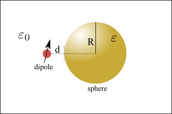
As is shown in above figure, In this project I will simulate the dipole’s emission near a sphere. The sphere could be dielectric or metalic. The theoretic description could be found in this paper ^ref1.

We will analyze two different types of dipole orientations.

• Radial dipole orientation which means dipole is orthogonal to the radial direction. $\mathrm{d}_{ort}$

• Tangential dipole orientation which means dipole is parallel to the radial direction. $\mathrm{d}_{para}$

  We will try to numerically and theoretically calculate the emission enhancement.

Theoretical Description

Theoretically, the total decay rate $\Gamma{t}$ and radiative decay rate $\Gamma{r}$ could be expressed as

• Radial Dipole

$$\begin{equation} \frac{\Gamma_{t}^{\bot}}{\Gamma_{0}}=1+\frac{3}{2}\text{Re}\sum_{l=1}^{\infty}(2l+1)l(l+1)b_{l}\left(\frac{h_{l}^{(1)}(kr)}{kr}\right)^2 \end{equation}$$ $$\begin{equation} \frac{\Gamma_{r}^{\bot}}{\Gamma_{0}}=\frac{3}{2}\text{Re}\sum_{l=1}^{\infty}(2l+1)l(l+1)b_{l}\left|\frac{j_{l}^{(1)}(kr)+b_{l}h_{l}^{(1)}(kr)}{kr}\right|^2 \end{equation}$$

• Tangential Dipole

$$\begin{equation} \frac{\Gamma_{t}^{\parallel}}{\Gamma_{0}}=1+\frac{3}{2}\sum_{l=1}^{\infty}(l+\frac{1}{2})\left[b_{l}\left(\frac{\xi_{l}^{\prime}(kr)}{kr}\right)^2+a_{l}(h_{l}^{(1)}(kr))^2\right) \end{equation}$$ $$\begin{equation} \frac{\Gamma_{r}^{\parallel}}{\Gamma_{0}}=\frac{3}{4}\sum_{l=1}^{\infty}(2l+1)\left[|j_{l}(kr)+a_{l}h_{l}^{(1)}(kr)|^2+\left|\frac{\psi^{\prime}(kr)+b_{l}\xi^{\prime}_{l}(kr)}{kr}\right|^2\right] \end{equation}$$

In above expressions, $j{n},h^{(1)}{n}$ are ordinary spherical Bessel and Hankel functions.

$$\begin{equation} \psi_{n}(x)\equiv xj_{n}(x),\quad \xi_{n}(x)\equiv xh^{(1)}_{n}(x) \end{equation}$$

$a{n}$ and $b{n}$ are the Mie scattering coefficients of the sphere. $r=R+d$, $k=\sqrt{\varepsilon}\omega/c$. $\varepsilon$ is the dielectric constant of the embedding medium, $\omega$ the optical frequency, $c$ the speed of the light in vacuum, and $l$ is the angular mode number. The derivatives of $\psi{n},\xi{n}$ are relatively to $kr$. The Mie scattering coefficients’ definition could be found in the book.^ref2

$$\begin{equation} a_{n}=\frac{\mu m^2j_{n}(mx)[xj_{n}(x)]^{'}-\mu_{1}j_{n}(x)[mxj_{n}(mx)]^{\prime}}{\mu m^2 j_{n}(mx)[xh^{(1)(x)}]'-\mu_{1}h_{n}^{(1)}[mxj_{n}(mx)]^{\prime}} \end{equation}$$ $$\begin{equation} b_{n}=\frac{\mu_{1} j_{n}(m x)\left[x j_{n}(x)\right]^{\prime}-\mu j_{n}(x)\left[m x j_{n}(m x)\right]^{\prime}}{\mu_{1} j_{n}(m x)\left[x h_{n}^{(1)}(x)\right]^{\prime}-\mu h_{n}^{(1)}(x)\left[m x j_{n}(m x)\right]^{\prime}} \end{equation}$$

MATLAB Implementation

I wrote an MATLAB program to realize the simulation of the emission enhancement. The following is the function and these function should be renamed and stored with a proper name according to the function name.

Function Program

% Main Function
function nP=Fun_nP_Cal(num_sum,num_dis,dis,alpha,alpham,index_s,k)
nP=zeros(num_dis,2); % with nP(:,1) store the np_ortho and nP(:,2) store the np_para
for m=1:num_dis
	rate_ortho=0;
    rate_para=0;
    r=dis(m);
	for l=1:num_sum
        a1=(index_s^2*spBJ(l,alpham)*dspBJ(l,alpha)-spBJ(l,alpha)*dspBJ(l,alpham));
        a2=(index_s^2*spBJ(l,alpham)*dspBH(l,alpha)-spBH(l,alpha)*dspBJ(l,alpham));   
        b1=(spBJ(l,alpham)*dspBJ(l,alpha)-spBJ(l,alpha)*dspBJ(l,alpham));
        b2=(spBJ(l,alpham)*dspBH(l,alpha)-spBH(l,alpha)*dspBJ(l,alpham));
	    x=k*r;
	    al=a1/a2;
	    bl=b1/b2;
		rate_ortho=rate_ortho+(2*l+1)*l*(l+1)*(-al)*(spBH(l,x)/(x))^2;
	    rate_para=rate_para+(l+0.5)*((-al)*(dspBH(l,x)/(x))^2+(-bl)*(spBH(l,x))^2);   
	end
	rate_ortho=real(rate_ortho)*3/2+1;
	rate_para=1+1.5*real(rate_para);
	nP(m,1)=rate_ortho;
	nP(m,2)=rate_para; 
end
end

% The Sphere Hankel Function of the first kind
function [spBH]=spBH(l,x)
    l=l+0.5;
    spBH=sqrt(pi/(x*2))*(besselj(l,x)+1j*bessely(l,x));
end

% The Sphere Bessel Function 
function [spBJ]=spBJ(l,x)
    l=l+0.5;
    spBJ=sqrt(pi/(x*2))*besselj(l,x);
end

% The derivative of the Hankel function of the first kind
function [dspBH]=dspBH(l,x)
    l=l+0.5;
    spBH1=sqrt(pi/(x*2))*(besselj(l,x)+1j*bessely(l,x));
    spBH2=sqrt(pi/(x*2))*(besselj(l-1,x)+1j*bessely(l-1,x));
    spBH3=sqrt(pi/(x*2))*(besselj(l+1,x)+1j*bessely(l+1,x));
    dspBH=0.5*spBH1+x*0.5*(spBH2-spBH3);
end

% The derivative of [the Hankel function of the first kind * mx]
function [dspBHm]=dspBHm(l,x)
    l=l+0.5;
    m=sqrt(-50);
    spBH1=sqrt(pi/(x*2))*(besselj(l,x)+1j*bessely(l,x));
    spBH2=sqrt(pi/(x*2))*(besselj(l-1,x)+1j*bessely(l-1,x));
    spBH3=sqrt(pi/(x*2))*(besselj(l+1,x)+1j*bessely(l+1,x));
    dspBHm=m*0.5*spBH1+x*0.5*(spBH2-spBH3);
end

% The derivative of the Bessel function
function [dspBJ]=dspBJ(l,x)
    l=l+0.5;
    spBJ1=sqrt(pi/(x*2))*besselj(l,x);
    spBJ2=sqrt(pi/(x*2))*besselj(l-1,x);
    spBJ3=sqrt(pi/(x*2))*besselj(l+1,x);
    dspBJ=0.5*spBJ1+x*0.5*(spBJ2-spBJ3);
end

% The derivative of [the Bessel function *mx]
function [dspBJm]=dspBJm(l,x)
    l=l+0.5;
    m=sqrt(-50);
    spBJ1=sqrt(pi/(x*2))*besselj(l,x);
    spBJ2=sqrt(pi/(x*2))*besselj(l-1,x);
    spBJ3=sqrt(pi/(x*2))*besselj(l+1,x);
    dspBJm=m*0.5*spBJ1+m^2*x*0.5*(spBJ2-spBJ3);
end

Main Program (Convergence Test)

And the main program is as follows

% To test when will the theoretical expressions will convengent
%index_s=sqrt(-22.473-1.3974i);
index_s=sqrt(-50);
lamda=1000e-9;
k0=2*pi/lamda;
k=k0;
radius=110e-9;
alpha=pi*2*radius/lamda;
alpham=alpha*index_s;
num_dis=100;

num_sum=[1,3,50];
num_len=length(num_sum);
dis_theo=linspace(radius+50e-9,radius+1000e-9,num_dis);

np_theo=zeros(num_dis,2,3);

for l=1:num_len
    np_theo(:,:,l)=Fun_nP_Cal(num_sum(l),num_dis,dis_theo,alpha,alpham,index_s,k);
end

%% 
figure(1)
for l=1:num_len
    plot(dis_theo,np_theo(:,1,l),'-')
    hold on
    plot(dis_theo,np_theo(:,2,l),'--')
end

Python Implementation

I also write a corresponding python program to calculate the dipole’s emission near sphere.

Simulation Methods

COMSOL Simulation

Dipole’s emission properties near nano particles could be simulated via COMSOL. COMSOL supports different types of sources, for example, the point, edge, surface and volume current source. The emission power could be described by

$$\begin{equation} \frac{\mathrm{d}W}{\mathrm{d}t}=\int_{s}\langle \vec{S}\rangle\cdot \boldsymbol{n}\mathrm{d}S=-\frac{1}{2}\text{Re}\int_{V} (J^{*}\cdot \boldsymbol{E})dV=\frac{\Omega}{2}\text{Im}(\boldsymbol{d}^{*}\cdot \boldsymbol{E}) \end{equation}$$

to be continued…….

MEEP Simulation

Lumerical FDTD Simulations

^ref1. Phys. Rev. B 76, 115123 (2007) ↩

^ref2. Absorption and scattering by small particles ↩