Neural Networks Learning I -Recognize Handwritten Digits
Python #Deeplearning
This is the beginning of my neural networks learning. I have read the books written by Michael Nielsen for a long time and I think now it’s time to complete the learning examples in first chapter of his book.

Introduction of some functions
I first want to show the use of some functions in his program example. These uses really surprise me a lot.
numpy.random
The first function is the random function from the package numpy. In initialize the matrix, the random function is used.
random.randn
Return a sample (or samples) from the “standard normal” distribution.
If positive, int_like or int-convertible arguments are provided, randn generates an array of shape (d0, d1, …, dn), filled with random floats sampled from a univariate “normal” (Gaussian) distribution of mean 0 and variance 1 (if any of the d_i are floats, they are first converted to integers by truncation). A single float randomly sampled from the distribution is returned if no argument is provided
1 | import numpy as np |
[0.34894831]
1 | print(np.random.randn(3)) |
[0.34444932 0.12172097 1.14900238]
1 | print(np.random.randn(2,3)) |
[[ 0.49635216 0.22762119 -0.68270641]
[-2.13526944 -0.82040908 -0.79356388]]
Random.shuffle
Modify a sequence in-place by shuffling its contents.
This function only shuffles the array along the first axis of a multi-dimensional array. The order of sub-arrays is changed but their contents remains the same.
1 | A=np.random.randn(4,4) |
1 | print(A) |
[[ 0.89532715 -2.34406351 -0.47233016 -0.1943856 ]
[ 0.57509425 -0.84810353 1.11576561 1.33146725]
[ 0.81883264 2.25208295 -1.52527099 -1.30444846]
[ 1.94464225 0.29825984 -0.16625868 -0.35876162]]
1 | np.random.shuffle(A) |
[[ 1.94464225 0.29825984 -0.16625868 -0.35876162]
[ 0.57509425 -0.84810353 1.11576561 1.33146725]
[ 0.81883264 2.25208295 -1.52527099 -1.30444846]
[ 0.89532715 -2.34406351 -0.47233016 -0.1943856 ]]
zip()
Python’s zip() function creates an iterator that will aggregate elements from two or more iterables. You can use the resulting iterator to quickly and consistently solve common programming problems, like creating dictionaries. In this tutorial, you’ll discover the logic behind the Python zip() function and how you can use it to solve real-world problems.
1 | A=['1','2','3'] |
<zip object at 0x000001D6AB168A08>
1 | type(ABC) |
zip
1 | list(ABC) |
[('1', 'A', 1), ('2', 'B', 2), ('3', 'C', 3)]
Matrix use
1 | A=np.array([1,2,3,4,5,6,7]) |
2
3
4
5
6
7
1 | for l in A[:-1]: |
1
2
3
4
5
6
1 | sizes=[2,3,4] |
1 | print(W) |
[array([[-0.53071848, -0.26905161],
[-0.75696575, -0.57292324],
[-1.47093334, 0.060232 ]]), array([[ 1.03193319, 0.58177683, 0.78046451],
[ 0.14132843, -0.90416154, -0.12645047],
[ 1.90204955, -0.55866015, 0.39481778],
[-0.11897701, 1.1277029 , 0.7584795 ]])]
My understanding on the neural networks
How we map the input to the output
Previously, I have learned the use of some special functions, now it’s time to give a summary of my understanding. I will not list everything since Michael Nieslen gives wonderful descriptions.
In my view, our problem is that we have a input which is usually a one dimensional array, the output is still an array. What we need do is to map the input to the output correctly.
In real life we will can describe and measure the world in different way. The color, the sound, the taste etc. However,
Anything is a number.
The properties in real world can all be mapped into a number space. And what happened in real world can be described by the numbers and number operations. For example, we use coordinate (x,y,z) to describe the position of the some object.
We create the neural networks and it has many layers. From the mathematical view, the input data
Where
So the value vectors in different layers will be linked with the the transformation. So this is how we obtain the output from the input.
In summary, we have a neural networks means we have a series of weight matrix and bias vectors. Different weights, bias, number of layers will give different neural networks. Our neural networks are actually a series of matrix, vectors.
How to measure the quality of the mapping?
To measure the quality of the mapping, we should compare the output data from our neural networks and the actual data. To measure the quality we can for example define the following cost function
If the difference between the output and the actual value is smaller, it means our neural networks works better.
How to train our neural networks?
A very important step of deep learning is to train our neural networks. Training means we change our weights and bias vector to let our output closer to the actual result.
To realize this, we need give some modifications after each learning. In machine learning, the down hill method is used to optimize our parameters. What we will do is just the same. The difference is that the effect of weights and bias on the output is more complex. We need choose a road in an abstract space to let the cost function decrease just like we go down in an abstract space.
So the partial derivative will be calculated. Some tricks will be used to let the change of the weight function and bias will always let the cost function decrease.
But what’s really exciting about the equation is that it lets us see how to choose
where
and the vector should be updated like this
However, for a neural networks, further derivation must be done to calculate the derivative of the weight and bias in each layers. Nielsen gives detailed explanation and proof.Back Propagation Method
Here is a simple summary,
The backpropagation equations provide us with a way of computing the gradient of the cost function. Let’s explicitly write this out in the form of an algorithm:
- Input x: Set the corresponding activation a1 for the input layer.
- Feedforward: For each l=2,3,…,L compute
and . - Output error
: Compute the vector . - Backpropagate the error: For each l=L−1,L−2,…,2 compute
. - Output: The gradient of the cost function is given by $\frac{\partial C}{\partial b{j}^{l}}=\delta{j}^{l}
\frac{\partial C}{\partial w{jk}^{l}}=a{k}^{l-1}\delta_{j}^{l}$.
Explanation of the program
Now I will focus on the program and give my own understanding of the function. I will follow the list of the program. The first is import necessary packages.
1 | """ |
Then the Sigmoid function and derivation of Sigmoid function will be defined.
1 | #### Miscellaneous functions |
Then a class named network will be defined. And in this class,the _init_ function is as follows1
2
3
4
5
6
7
8
9
10
11
12
13
14
15
16def __init__(self, sizes):
"""The list ``sizes`` contains the number of neurons in the
respective layers of the network. For example, if the list
was [2, 3, 1] then it would be a three-layer network, with the
first layer containing 2 neurons, the second layer 3 neurons,
and the third layer 1 neuron. The biases and weights for the
network are initialized randomly, using a Gaussian
distribution with mean 0, and variance 1. Note that the first
layer is assumed to be an input layer, and by convention we
won't set any biases for those neurons, since biases are only
ever used in computing the outputs from later layers."""
self.num_layers = len(sizes)
self.sizes = sizes
self.biases = [np.random.randn(y, 1) for y in sizes[1:]]
self.weights = [np.random.randn(y, x)
for x, y in zip(sizes[:-1], sizes[1:])]
Be careful the use of size[:-1],size[1:] which means the matrix removed the last element and last element respectively. The use of zip is also new to me and self.weights is constructed by a series of matrix with different dimensions.
The feedforward function that which update
1 | def feedforward(self, a): |
Here is the SGD main function
1 | def SGD(self, training_data, epochs, mini_batch_size, eta, |
The main training function. A test data will be used if needed. We give the training data which will be loaded use well defined function
1 | import mnist_loader |
This function will divide the step of training and show the progress and quality of the neural networks if we give the test data. The function update_mini_batch will update the weights and bias for a given training data.
update_mini_batch function is defined as follows
1 | def update_mini_batch(self, mini_batch, eta): |
The partial derivative for weights and biases will be defined first. Then the partial derivative will be calculated use the function backprop. And the new weights will bias will be updated. The most important part is the function backprop
1 | def backprop(self, x, y): |
This function is a realization of previous explanation of the back propagation methods. And finally, the two other functions
1 | def evaluate(self, test_data): |
which is very easy to understand.
How to use?
This is really a good example of neural networks deep learning. To use this, you can direct download Michael Nielsen’s example. However, he writes this use python2, to use python3, you can use the another example by MichalDanielDobrzanski
after downloading the repository, the file network.py is just like we shown above. The following is the use of the program
1 | C:\Users\xiail\Documents\Dropbox\Code\Python\Study\Neural-Networks\Study-1\DeepL |