Meep

说明

回归科研以后，一些爱好需要重新拾取起来了。最近学会了用COMSOL计算光子晶体能带，现在尝试来用Meep计算光子晶体能带，希望可以以后有机会作为主力的程序来使用。

我主要参考的是官方文档：https://mpb.readthedocs.io/en/latest/Python_Tutorial/

简单二维光子晶体能带例子

能带计算

本次主要想重复书籍Photonic Crystals: Molding the Flow of Light second edition 第五章的结构的能带计算：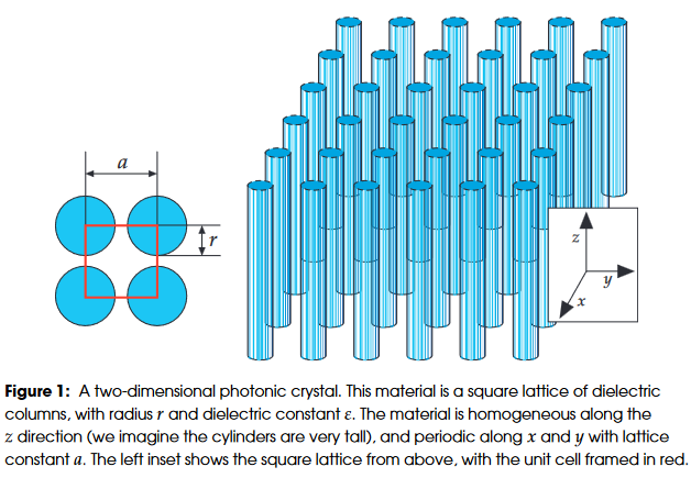

按照官方文档的介绍，直接设置结构，计算相应能带即可，具体可以看代码和注释

import math
import meep as mp
from meep import mpb

num_bands = 8

# 定义好扫描的k波矢
k_points = [mp.Vector3(),          # Gamma
            mp.Vector3(0.5),       # X
            mp.Vector3(0.5, 0.5),  # M
            mp.Vector3()]          # Gamma

# 对k波矢进行插值
k_points = mp.interpolate(20, k_points)

# 基本结构和材料性质
geometry = [mp.Cylinder(0.2, material=mp.Medium(epsilon=8.9))]

# 基本二维cell
geometry_lattice = mp.Lattice(size=mp.Vector3(1, 1))

resolution = 32

# mode solver设置
ms = mpb.ModeSolver(num_bands=num_bands,
                    k_points=k_points,
                    geometry=geometry,
                    geometry_lattice=geometry_lattice,
                    resolution=resolution)

# 计算te模式
print("Square lattice of rods: TE bands")
ms.run_te()

按照官方文档说法，要查看得到的本振频率，需要从输出的类似的log文件中提取，比如：

1	tefreqs:, 13, 0.3, 0.3, 0, 0.424264, 0.372604, 0.540287, 0.644083, 0.81406, 0.828135, 0.890673, 1.01328, 1.1124

我们需要手动将这些信息提取出来，在Linux里面主要通过正则表达式提取，这种方式感觉太不优雅了，官方文章还有例子MPBData：

1	tm_freqs = ms.all_freqs

所以可以直接从ms中提取结果

ms.run_te()
te_freqs = ms.all_freqs
te_gaps = ms.gap_list
ms.run_tm()
tm_freqs = ms.all_freqs
tm_gaps = ms.gap_list

可以将能带绘制出来

import matplotlib.pyplot as plt
numk,tmp=np.shape(te_freqs)
klist=range(numk)


fig,ax=plt.subplots()
x = range(len(tm_freqs))
  
for l in range(num_bands):
    plt.plot(te_freqs[:,l],'r-')
    plt.plot(tm_freqs[:,l],'b-')
plt.ylim([0,0.8])
plt.ylabel('$\omega a/(2\pi c)$')

# Plot gaps
for gap in tm_gaps:
    if gap[0] > 1:
        ax.fill_between(x, gap[1], gap[2], color='blue', alpha=0.2)

for gap in te_gaps:
    if gap[0] > 1:
        ax.fill_between(x, gap[1], gap[2], color='red', alpha=0.2)

  
points_in_between = (len(tm_freqs) - 4) / 3
tick_locs = [i*points_in_between+i for i in range(4)]
tick_labs = ['Γ', 'X', 'M', 'Γ']
ax.set_xticks(tick_locs)
ax.set_xticklabels(tick_labs, size=16)

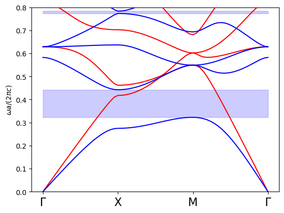
书中的结果是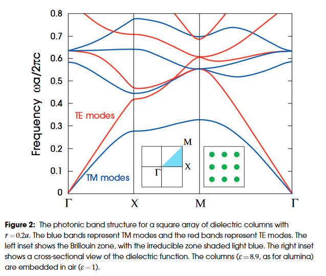

可以看到与书籍的结果是一样的。并且可以比较方便的导出Band Gap，还是比较方便的。

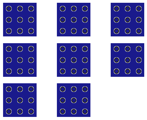
电场导出

以上是能带计算的例子，我们也可以导出相应的电场分布，观察tm模式的Ez，

efields = []
def get_efields(ms, band):
    efields.append(ms.get_efield(band, bloch_phase=True))

ms.run_tm(mpb.output_at_kpoint(mp.Vector3(1/2, 0,0), mpb.fix_efield_phase,
          get_efields))

# Create an MPBData instance to transform the efields
eps = ms.get_epsilon() # 得到折射率分布
md = mpb.MPBData(rectify=True, resolution=32, periods=3)
converted_eps = md.convert(eps) 

converted = []
for f in efields:
    # Get just the z component of the efields
    f = f[..., 0, 2]
    converted.append(md.convert(f))


for i, f in enumerate(converted):
    plt.subplot(331 + i)
    plt.contour(converted_eps.T, cmap='binary')
    plt.imshow(np.real(f).T, interpolation='spline36', cmap='jet', alpha=0.9)
    plt.axis('off')

plt.show()

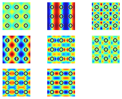
按道理应该没有Ex,Ey分量，可以进行测试,绘制一下Ex

# Create an MPBData instance to transform the efields
eps = ms.get_epsilon() # 得到折射率分布
md = mpb.MPBData(rectify=True, resolution=32, periods=3)
converted_eps = md.convert(eps)
  
converted = []
for f in efields:
    # Get just the  component of the efields
    f = f[..., 0, 0]
    converted.append(md.convert(f))

  
for i, f in enumerate(converted):
    plt.subplot(331 + i)
    plt.contour(converted_eps.T, cmap='binary')
    plt.imshow(np.real(f).T, interpolation='spline36', cmap='jet', alpha=0.9)
    plt.axis('off')


plt.show()