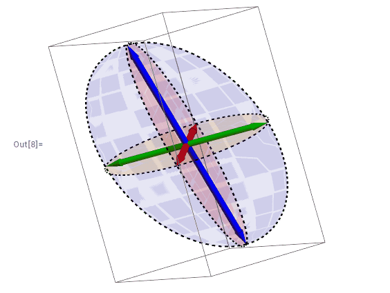
三维偶极取向:三维箭头的绘制
Mathematica
目的:
绘制给定直角坐标系下三个垂直的三维箭头,需要绘制出三维效果。
MATLAB没有天然的三维箭头绘制支持,需要用到别人写好的包。我经过多次尝试发现这些包的实现结果都不如人意。最后不得不采用Mathematica来实现,实现的过程中也发现有许多的坑,本篇笔记将会对实现方法进行记录。
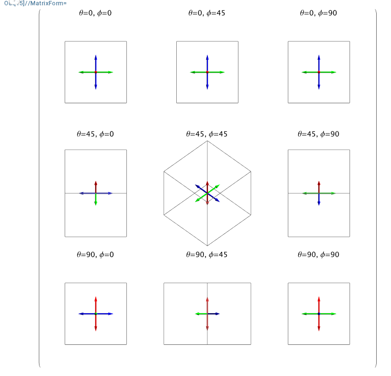
角度的对比
用Mathematica绘制时,1
2
3
4
5
6
7
8
9
10
11
12
13
14
15
16
17
18
19
20
21
22
23
24
25
26
27
28
29
30
31
32
33
34Table[
viewpt = {Sin[\[Theta]view]*Cos[\[Phi]view],
Sin[\[Theta]view]*Sin[\[Phi]view], Cos[\[Theta]view]};
Module[{ thickline = 0.02, thickhead = 0.05},
{d1, d2, d3} = Dipole3DfromRot[{1, 1, 0, 0, 0}];
p2 = Graphics3D[{(*Text[Style["d1",18,Red],d1],*)
{Red, Arrowheads[thickhead],
Arrow[Tube[{{0, 0, 0}, d1}, thickline]]}, {Red,
Arrowheads[thickhead],
Arrow[Tube[{{0, 0, 0}, -d1}, thickline]]},
(*Text[Style["d2",18,Red],d2],*)
{Green, Arrowheads[thickhead],
Arrow[Tube[{{0, 0, 0}, d2}, thickline]]}, {Green,
Arrowheads[thickhead],
Arrow[Tube[{{0, 0, 0}, -d2}, thickline]]},
(*Text[Style["d3",18,Red],d3],*)
{Blue, Arrowheads[thickhead],
Arrow[Tube[{{0, 0, 0}, d3}, thickline]]}, {Blue,
Arrowheads[thickhead],
Arrow[Tube[{{0, 0, 0}, -d3}, thickline]]}},
Boxed -> True, Axes -> False, AspectRatio -> 1,
AxesLabel -> {"X", "Y", "Z"},
PlotRange -> {{-1, 1}, {-1, 1}, {-1, 1}},
PlotLabel ->
"\[Theta]=" <> ToString[\[Theta]view/\[Pi]*180] <> ", \[Phi]=" <>
ToString[\[Phi]view/\[Pi]*180]];
pexport =
Show[p2, ViewPoint -> 3*viewpt, AspectRatio -> 1,
ViewProjection -> "Orthographic",
AxesOrigin -> {0, 0, 0}]], {\[Theta]view,
0, \[Pi]/2, \[Pi]/2/2}, {\[Phi]view,
0, \[Pi]/2, \[Pi]/2/2}] // MatrixForm
而采用MATLAB时,
1 | addpath('./FunctionFolder') |
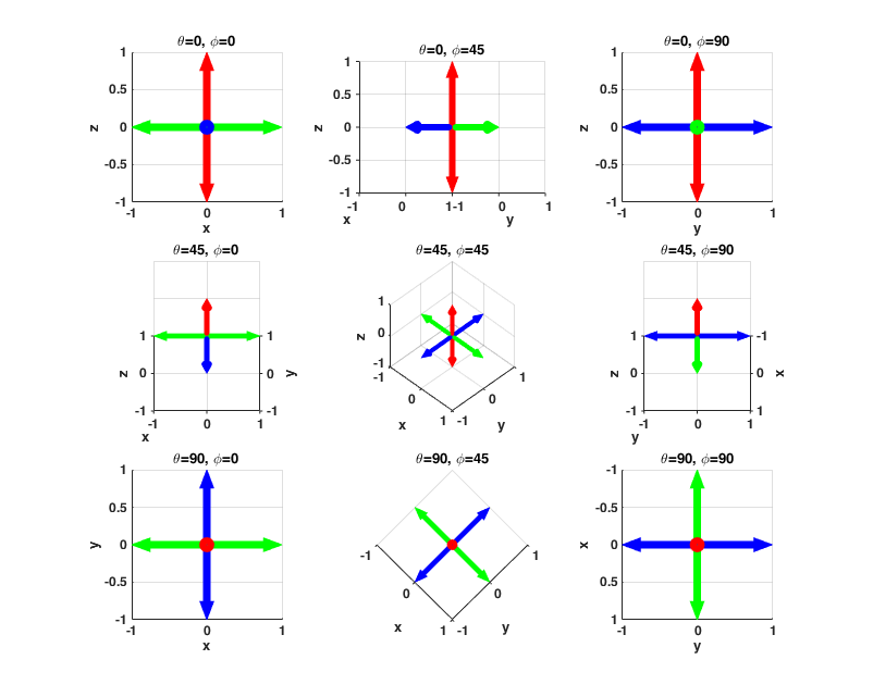
可以看见默认的角度是不一样的,为了角度一致,需要进行调制,变换规则为
调整以后就可以了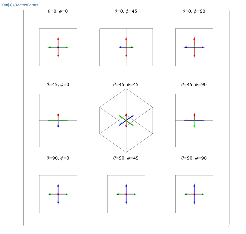
在三个箭头中添加椭圆
还需要添加相应的椭圆,这里设计到三维空间中椭圆的绘制。1
2
3
4
5
6
7
8
9
10
11
12
13
14
15
16
17
18
19
20
21
22
23
24
25
26
27
28
29
30
31
32
33
34
35
36
37
38
39
40
41
42
43
44
45
46
47
48
49
50
51
52
53
54
55
56
57
58
59
60
61
62
63
64
65
66
67
68
69
70
71
72
73
74
75
76
77
78
79
80
81
82
83
84
85
86
87
88
89
90
91
92
93parafit = {2, 3, 1, 2, 3};
\[Theta]view = \[Pi]/2; \[Phi]view = \[Pi]/2;
viewpt = {Sin[\[Theta]view]*Cos[\[Phi]view],
Sin[\[Theta]view]*Sin[\[Phi]view], Cos[\[Theta]view]};
Module[{\[Alpha] = parafit[[1]], \[Beta] = parafit[[2]],
thickline = 0.02, thickhead = 0.05},
dx = N[{1, 0, 0}];
dy = N[{0, \[Alpha], 0}];
dz = N[{0, 0, \[Beta]}];
{d1, d2, d3} = Dipole3DfromRot[parafit];
d1D = Flatten[{d1, d2, d3}];
dxyz = {Flatten[{dx, dx*0, dx*0}], Flatten[{dx*0, dx, dx*0}],
Flatten[{dx*0, dx*0, dx}],
Flatten[{dy, dy*0, dy*0}], Flatten[{dy*0, dy, dy*0}],
Flatten[{dy*0, dy*0, dy}],
Flatten[{dz, dz*0, dz*0}], Flatten[{dz*0, dz, dz*0}],
Flatten[{dz*0, dz*0, dz}]};
M1D = Inverse[dxyz] . d1D;
M = ArrayReshape[M1D, {3, 3}];
p1 = ParametricPlot3D[
M . {Sin[\[Theta]]*Cos[\[Phi]], \[Alpha]*Sin[\[Theta]]*
Sin[\[Phi]], \[Beta]*Cos[\[Theta]]}, {\[Theta],
0, \[Pi]}, {\[Phi], 0, 2*\[Pi]}, Mesh -> None,
PlotStyle ->
Directive[Yellow, Opacity[0.1], Specularity[White, 20]],
Axes -> False , Boxed -> False];
p1cut =
ParametricPlot3D[
M . {Sin[\[Theta]]*Cos[\[Phi]], \[Alpha]*Sin[\[Theta]]*Sin[\[Phi]],
0*Cos[\[Theta]]}, {\[Theta], 0, \[Pi]}, {\[Phi], 0, 2*\[Pi]},
Mesh -> None,
PlotStyle ->
Directive[RGBColor[1, 1, 0], Opacity[0.1], Specularity[White, 20]],
Axes -> False , Boxed -> False];
p2cut =
ParametricPlot3D[
M . {Sin[\[Theta]]*Cos[\[Phi]],
0*Sin[\[Theta]]*Sin[\[Phi]], \[Beta]*Cos[\[Theta]]}, {\[Theta],
0, \[Pi]}, {\[Phi], 0, 2*\[Pi]}, Mesh -> None,
PlotStyle ->
Directive[RGBColor[1, 0, 0], Opacity[0.1], Specularity[White, 20]],
Axes -> False , Boxed -> False];
p3cut =
ParametricPlot3D[
M . {Sin[\[Theta]]*Cos[\[Phi]]*0, \[Alpha]*Sin[\[Theta]]*
Sin[\[Phi]], \[Beta]*Cos[\[Theta]]}, {\[Theta],
0, \[Pi]}, {\[Phi], 0, 2*\[Pi]}, Mesh -> None,
PlotStyle ->
Directive[RGBColor[0, 0, 1], Opacity[0.1], Specularity[White, 20]],
Axes -> False , Boxed -> False];
p1Cir1 =
ParametricPlot3D[
M . {Cos[\[Phi]], \[Alpha]*Sin[\[Phi]], 0}, {\[Phi], 0, 2*\[Pi]},
PlotStyle ->
Directive[Dashed, Black, Opacity[1], Specularity[White, 20],
Thickness[0.005]],
Axes -> False , Boxed -> False];
p1Cir2 =
ParametricPlot3D[
M . {Sin[\[Theta]], 0, \[Beta]*Cos[\[Theta]]}, {\[Theta], 0,
2*\[Pi]},
PlotStyle ->
Directive[Dashed, Black, Opacity[1], Specularity[White, 20]],
Axes -> False , Boxed -> False];
p1Cir3 =
ParametricPlot3D[
M . {0, Sin[\[Theta]]*\[Alpha], \[Beta]*Cos[\[Theta]]}, {\[Theta],
0, 2*\[Pi]},
PlotStyle ->
Directive[Dashed, Black, Opacity[1], Specularity[White, 20]],
Axes -> True , Boxed -> True];
p2 = Graphics3D[{(*Text[Style["d1",18,Red],d1],*)
{Red, Arrowheads[thickhead],
Arrow[Tube[{{0, 0, 0}, d1}, thickline]]}, {Red,
Arrowheads[thickhead],
Arrow[Tube[{{0, 0, 0}, -d1}, thickline]]},
(*Text[Style["d2",18,Red],d2],*)
{Green, Arrowheads[thickhead],
Arrow[Tube[{{0, 0, 0}, d2}, thickline]]}, {Green,
Arrowheads[thickhead],
Arrow[Tube[{{0, 0, 0}, -d2}, thickline]]},
(*Text[Style["d3",18,Red],d3],*)
{Blue, Arrowheads[thickhead],
Arrow[Tube[{{0, 0, 0}, d3}, thickline]]}, {Blue,
Arrowheads[thickhead], Arrow[Tube[{{0, 0, 0}, -d3}, thickline]]}},
Boxed -> True];
pexport =
Show[(*p1,*)p2, p1Cir1, p1Cir2, p1Cir3, p1cut, p2cut, p3cut, p2(*,
ViewPoint\[Rule]34*viewpt*), AspectRatio -> 1,
ViewProjection -> "Orthographic", AxesOrigin -> {0, 0, 0},
Lighting -> Automatic]]